Numeric Integration
Objectives
- Practice writing Python functions.
- Gain experience with list comprehensions.
- Write helper functions and compose large functions from smaller ones.
Background
In this lab you will build a python program that can compute the areas underneath arbitrary mathematical functions (mathematicians call these integrals). In addition, you’ll calculate answers that mathematicians don’t have formulas for…and you’ll never have to use anything more complicated than multiplication!
Getting started…
Start by creating a new file, we will call ours integrals.py, and pasting this code into it:
Trying out list comprehensions
To begin, try out list comprehensions at the Python prompt… these examples should help build intuition about how list comprehensions work:
Read over those three one-line functions; be sure you have internalized how they work!
Note that the calls lc_idiv(10) and lc_fdiv(10) return different lists; the first uses integer division (rounding down); the second uses floating-point division.
Integration: why? and what?
Integration is sometimes described as finding the area between a mathematical function and the horizontal (x) axis.
More generally, integration is simply the sum of a numeric function’s results, i.e., y-values across a chosen span.
It is important because it provides a one-number summary of what the function is “doing” over an interval. It’s also used to determine how fields of forces act on a particular point, surface, or object over time; it is also essential in defining a function’s “average value” on an interval or region. Integrals can be used to design an airplane wing, predict the weather, or calculate how much a bank account will be worth in ten years even if interest rates are changing.
As an example, recall the dbl function from above (with a better docstring):
This function could be written algebraically as y = 2x, where y is the functions return value and x is its input.
Suppose you wanted to estimate the integral of dbl, on the interval between 0.0 and 10.0. You could create the following (rough) approximation with rectangles:
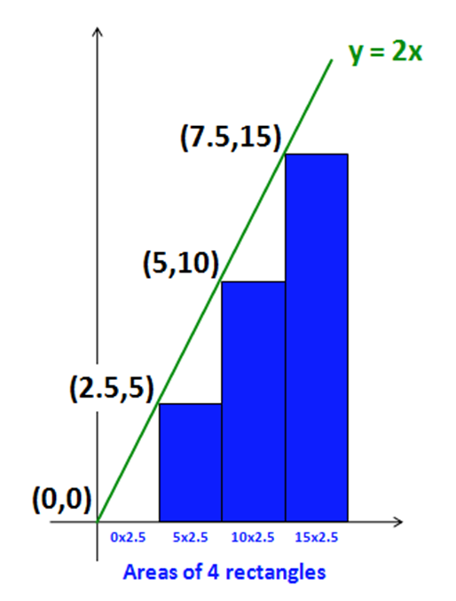
- Here, the interval is divided into 4 parts. The list
[0, 2.5, 5, 7.5]contains eachxvalue of the left-hand endpoint of each of the four subintervals. - We next find the return values from
dbl(x)for each possiblexin the list above. Here, we name these return valuesy. The list of these values is[0, 5, 10, 15]. - Now we add up the areas of the rectangles whose upper-left-hand corner (height) is at these
yvalues. Each rectangle extends down to thex-axis. Each rectangle’s individual width is 2.5, because there are four equal-width rectangles spanning a total of 10 units of width. - We find the rectangles’ areas in the usual way. Their heights are contained in the list
yand their widths are 2.5, so the total area is0*2.5 + 5*2.5 + 10*2.5 + 15*2.5or(0 + 5 + 10 + 15)*2.5which is(30)*2.5, or75.
Yes, this is a very rough approximation for the “area under the curve,” i.e., the integral. But if we make the width of the rectangles smaller, their sum will approximate that area as closely as we’d like!
More importantly, this example suggests a general way to approximate a function’s integral over a known interval:
- Divide the interval into
Nequal parts and create a list with the correspondingx(argument) values. - Find the
yvalues (results) of the function for each value ofxcalculated in step 1 - Calculate the area of each rectangle under the curve. Their heights are the
yvalues; their widths are the separation between thexvalues. - Sum the rectangles’ areas and return the result: that’s the integral, or an approximation that can be made arbitrarily close by adding more rectangles.
The rest of this exercise involves writing functions for each of these four steps; then you’ll use those functions to answer questions about the results.
Step 1: Calculating the x values to be evaluated
First, you will write a function named unitfracs(N) and then one named scaledfracs(low, hi, N).
Writing unitfracs…
Writing unitfracs …
Take a look at how unitfracs(N) works:
To do: Write
unitfracs(N).As its name suggests, it returns a list of evenly-spaced left-hand endpoints (fractions) in the unit interval [0, 1).
Copy, paste, and alter the example function lc_fdiv in order to write unitfracs. You will only need to change a single character from that code!
Be sure to write the docstring of
unitfracsto reflect what it does, as well.And finally, write at least three
assertstatements that implement tests for some of the examples above.
Writing scaledfracs…
Next, take a look at how scaledfracs(low, hi, N) works:
To do: Write
scaledfracs(low, hi, N). It createsNleft endpoints uniformly through the interval [low, hi).Again, write assert statements to test the examples above.
This is tricky … here is some additional explanation:
Use unitfracs. For example, use this line as a starting point:
return [ for x in unitfracs(N)]
This way, you won’t have to redo the work of unitfracs!
You might feel that this is closely related to the interp function you wrote before—you’re right!
You don’t need to use that interp function, but you will want to use the ideas from it! Here it is, for reference:
Note that the role of
fracabove is as the “interpolating fraction,” which is exactly whatxis doing in the list comprehension!Do include a docstring that reflects what
scaledfracsdoes.
Step 2: Calculating the y values
Your scaledfracs function can produce arbitrary lists of evenly-spaced x values.
Next, you’ll need to calculate the y values (results) of a function at each of these x positions. Again, you’ll use list comprehensions to make this process simple and fast!
Although the goal is to handle arbitrary functions, we’ll start with a concrete function and build up.
Writing sqfracs…
To do: Write a function
sqfracs(low, hi, N)that works as follows:
Here,
sqfracsis very similar toscaledfracsexcept that each value is squared.
Use scaledfracs here. In the same way that scaledfracs used unitfracs, sqfracs can use scaledfracs! Consider the snippet:
for x in scaledfracs(low, hi, N)
{
asserts to test sqfracs. For extra fun, concoct some additional examples of your own!Writing f_of_fracs…
To do: Write a function
f_of_fracs(f, low, hi, N)that works as follows:
Note that
f_of_fracstakes a function as its first argument—this is no problem inpython.You might copy and paste
sqfracsas a model: only a few characters need to be changed! (You only need 3 keystrokes to fix this one!)The third example above is tricky to test with assert—it can be done, but it’s hard to do properly. Note that it’s not correct to run
f_of_fracs(sin, ...)and then copy its output into anassertstatement: in that case you would be saying “the right answer is the one my function calculated, even if my function got the wrong answer!”
Step 3: Calculate the area and put it all together
You now have functions that calculate both the x and, more importantly, the y values of a function at regularly-spaced intervals. Well done! Now we just have to put it all together.
To do: Write
integrate(f, low, hi, N)which will return the final, desired value: the integral offfromlowtohiusingNsteps.Take a look at a few examples and hints below.
As these examples highlight,
integratedoes not return a list; it returns a single, floating-point value:
Don’t worry about small errors in the rightmost (least-significant) digits. They occur from small differences in
pythonversions.To get started, here is the “signature” (the def line) and docstring for integrate. Feel free to use this:
This time, we’ll try “test-driven development”, in which you write the tests first and then make your function satisfy the tests. That’s why we included the asserts above! (Note that the second assert is an example of how to test even if you don’t know the numerical answer!)
Do NOT use a list comprehension: no list is being created here. Rather, use f_of_fracs to generate the list of heights you need. Remember that the result of f_of_fracs is a big list of y-values! You want to multiply those y-values (heights) by the rectangles’ width. But all the widths are the same! So, you can sum the heights then multiply by the width! Use python’s built-in sum. sum(L) returns the sum of the elements in the list L.
Some examples of how sum works:
If your
integratefunction works, congratulations! You’ve built a general-purpose routine that can provide integrals for any computable function (including those for which there is no closed-form integral—i.e., ones where the best mathematicians in the world don’t know how to compute an exact result).